Crowd Dynamics
Motivation
So in my third semester one of my Fluid Mechanics professor Prof. Naveen Tiwari taught us ESO204, which is an introductory course on fluid mechanics. And after studying that course, I also watched the lectures of Prof. Sanjay Mittal, who supervised me in this project in crowd dynamics. I watched his lectures on YouTube, and I loved those lectures. In the course, however, Professor Naveen Tiwari also mentioned that "Fluid could also be used to model crowds," and that sentence kind of stuck with me. Because when studying fluid, if someone tells you what you are studying is also how crowds behave, you may be left thinking about this idea. It was very intriguing for me to think about people as particles of fluid. And I kind of thought it is not at all a bad way to compare. I mean, when in a dense crowd, I could imagine that I really don't have any control over myself (just like fluid). By which I mean, one loses his individuality and just goes where the crowd takes it. Just like the fluid flowing.
About a year later, I happened to go to a Jyotirlinga temple in Omkareshwar, in Madhya Pradesh, where I truly experienced the crowd in its true sense. I mean, as far as I could remember, this might be the most brutal crowd I had ever experienced. That was the first trigger point which led me to crowd dynamics. Later in the summer of 2025, I thought of working in this field, and got to know that there are different softwares made to simulate the flow of crowd in microscopic point of view, (meaning to model each pedestrian individually). But I found the papers back then to be a bit difficult. So I thought maybe this is not the time for me to work on this.
Then during the add-drop period (which is the period where students could add or drop a course during the registration in a semester), I found that we had a UGP (Undergraduate Project) in our template in the 7th semester. And this gave me another hope to start my work in crowd dynamics. And then I met Prof. Sanjay Mittal and discussed with him these ideas. I knew that he had worked in the feild of traffic flows, which is similar to crowd dynamics, but for vehicles and traffic.
Meeting 1
Meeting 1
The first meeting was about formulating the problem. Back then I found that formulating the problem itself is the most difficult part of the project. I came up with some very bizarre ideas like simulating the crowd on the path of temples and seeing how the people moved in the twisty paths of temples, etc. After the discussion, I was very clear that "Just because I want to do something doesn't mean that I should straight away start doing it". Now if I think about all that, I ask myself what I really wanted to do? I mean, I could simulate the crowd, but then what? So I found that I lacked a clear objective.
I was given the following paper and told to come up with a clear objective.
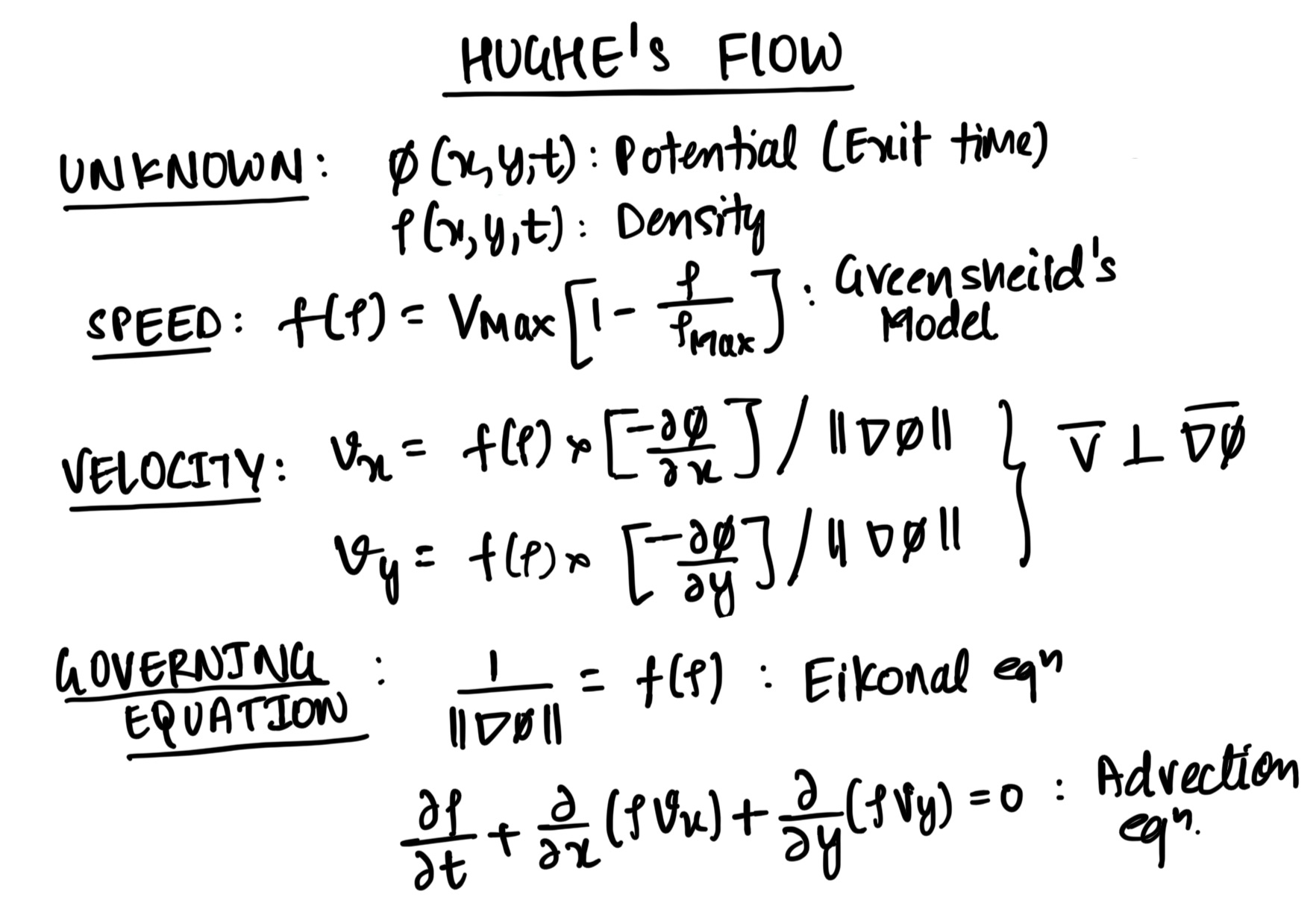
Here are the papers : Traffic Flows, Hughe's Flow
These were the paper suggested.
Meeting 2
Meeting 2
In this section I finally made the big move, and here is my First Report that I made. This was made after we had a discussion on the traffic flows, and how we could relate the traffic flow with crowd dynamics. Now this still needed somewhat discussion. Reading through the report, I feel I was still a naive thinker. My objectives were still not satisfactory. But one thing that I need to specify is that I still feel that the second objective has some potential. I mean, this idea (which was also suggested by Professor) came from the understanding that the flow moving through a CD nozzle will choke at some point. And therefore sir said that "If there is one pedestrian moving into the entrance there is no problem, and everyone entering will have absolutely no problem in moving through the paths. But if there are all the people jammed inside the path, we see no motion of people. So there must be a value of inflow rate of people where something like choking must be happening." Even till now when Meeting 7 has been done, I still think that this is a good subject.
Here is one more paper that porfessor recommnended, Here
This was said to me as a paper that has implements the hughe;s flow numerically.
Meeting 3
Meeting 3
So in the next week I made the This report. And this was the first turning point in my project. I implemented my first code for the hughe's flow. Although it wasn't that good but was considerable amount of progress.
Here are the results:
The results to me looked very senseless, but nevertheless at least I had something. Since my results made no sense, I now had to do the following. I had to validate the methods that I have used in this project, and this includes the Fast Sweep Method and the method used for advection. So for the advection, I have used the simple upwinding, and to validate the fast sweep I decided to replicate and spend some time understanding the eikonal equation. I have used this paper for that. So now the objective for my next lab was to work on the FAST SWEEP METHOD. Also, in the fast sweep, they have tried using the distance function, so for that, I read about this paper about the distance equation. Here
Meeting 4
Meeting 4
Here is the Report_1 (Hughe's Flow) and Report_2 (Eikonal Equation) for this meeting that I made. And here my task was to use some synthetic function and use it to test how good the algorithm is to solve the Eikonal equation. And so I did the same as mentioned in the paper. But one problem was that I checked the validity of this algorithm on a problem that contained Dirichlet condition on the boundary, which was not the case with my project. So this gave me the objective for my next lab that is to apply the well posed Neumann boundary condition on the problem and then use the algorithm in the main Hughe's flow solver. He tried to explain that using an algorithm that we don't fully understand should not be used until it is fully validated. So now my next task was to again validate the fast sweep method but this time for Neumann condition.
In addition to that I was also asked to make a toy problem and see if the advection equation is really working. So what he tried explaining me was that "If I am unable to solve the problem all at once, try breaking it into fragments (which is advection and fast sweep) and see if they work fine individually."
Shown below are some results:
Meeting 5
Meeting 5
Here is the Report 1 (Hughe's Flow) and Report 2 (Fast Sweep Method) of this meeting. Here I realised that the paper doesn't really discuss about implementing the FAST SWEEP METHOD on the problems containing Neumann boundary condition. And thus this needs to be fixed. As mentioned in the paper, I used the Ghost point approach and somehow tried coming up with the solution, and then used that understanding of fast sweep into Hughe's flow solver.
So now I was implementing Lax Wendroff scheme for advection because what I saw was that first order upwinding scheme had lots of numeric diffusion, and the Lax Wendroff was better in all the sense except that it had many numerical oscillations that were explained to be Gibbs oscillation occurring due to sharp discontinuity at the tip of discontinuity (Fourier transformation). And the results were also not very appreciable. They still looked like something really wrong is going on with them. And then the suggestion was "Why not start with a simple one dimensional problem and then see if it's working. It will be easier to study one dimensional flow compared to two dimensional." And so the next task was to simulate the Hughe's flow in one dimension.
Meeting 6
Meeting 6
Here is the Here of my progress.
Now at the first instant I thought I still messed up the problem. I used the ghost point approach to implement Neumann condition on \(\phi\) while solving Eikonal equation using Fast Sweep Method. And while doing so I also implemented Lax Wendroff scheme for advection in the density. The results were not very good, and I still was not at all satisfied.
Here are the results for your understanding
/Initial_Density_Distribution.png)
All of these didn't go well, and there were some problem that professor said me about :
- The initial condition taken was not at all good. Since I have been for all this time taking the initial condition containing sharp discontinuities in the density. And since my problem contained shocks due to non linear advection equation with velocity proportional to negative of density, sir said it would be better to pick the boundary condition which was too close to the minimum or maximum value of density.
- Also I was trimming the density if it ever exceeded the maximum value, this seemed to cause problem since in that case I would be solving a very different problem all together.
After making the changes in the initial condition all of a sudden the result started to make sense. A boundary condition of \(\rho = 0\) at the boundary for no inflow and the formation of shock due to crowd behind the peak having higher velocity, all of it was working just fine. Given below are the results
This made it clear that the problem was in the type of intial condition I was implementing really, and not in anything else. So now it was about extending to two dimension, from where I came.
Meeting 7
Meeting 7
Now it was about making the two dimensional flows. And here is the Report
Here I went in all the direction and tried many different problems. given below are all the problems :
| Problem | Initial Condition | Density | Potential | Velocity |
|---|---|---|---|---|
| Standard Exmaple |
/Standard_Example/IMG_20251017_001838.jpg)
|
|||
| Two Blob |
|
|||
| Unsymmetrical Exit |
|
|||
| Multi-Exit Problem - 1 |
/Multi_Exit_Problem_1/IMG_20251017_002514.jpg)
|
|||
| Multi-Exit problem |
/Multi_Exit_Problem_2/IMG_20251017_003527.jpg)
|
After the meeting there were two things that came into notice. That the boundary condition on density was not being respected, and also professor said me to compare the solution with some paper that actually solves a problem of Hughe's flow, because this might be helpful to validate the methods I am using to solve the problem. And so my next task was to replicate the result of This paper.
Meeting 8
Meeting 8
This work is based on a paper employing WENO schemes, using a third-order WENO fast sweeping method to solve the Eikonal equation and a fifth-order WENO scheme for the density advection equation; these are highly sophisticated numerical methods, and the problem further involves an internal obstacle whose accurate numerical modeling is non-trivial, with the exact implementation detailed in this report, while the reference paper can be found here.
Using the method for modelling the obstacle I tried some of my own problems out of curiosity an dthye are shown below.
| Problem | Density | Potential |
|---|---|---|
| Obstacle 1 | ||
| Obstacle 2 | ||
| Intelligent Crowd |
And looking at the results I am not at all disappointed. At least all the result made sense. Just the boundary condition has to be taken care of later.
So with that understanding I tried implementing the exact same problem which was done in the paper, and the result of which are shown below. When comparing them with that of the paper, they were not at all similar. The results in paper was very different. And following were the problem that we thought.
And looking at the results I am not at all disappointed. At least all the results made sense. Just the boundary condition has to be taken care of later.
So with that understanding I tried implementing the exact same problem which was done in the paper, and the results of which are shown below. When comparing them with that of the paper, they were not at all similar. The results in the paper were very different. And the following were the problems that we thought of.
- The paper used 5th order method which had much higher accuracy and resolution compared to my first order method. This was also suggested by the professor.
- Secondly I knew that I am not respecting the boundary condition when solving the problem, especially at the obstacle, and this was also a source of problem.
- And lastly, the problem took into account the Discomfort Factor \(g(\rho(x,y,t),x,y,t)\), but I kept it to be one. This was mentioned in the Hughes' paper that it could be taken as unity.
Here are the results:
Now the task was to really use the exact same scheme used in the paper and use it replicate the result of the paper.
Meeting 9
Meeting 9
This I consider to be the final meeting with the professor, and I believe I will have to really perform well this time. So here is the research paper that I will be using.
The task in today's attempt is to use the same method as used in the research paper, and kind of replicate the results. So that includes learning about the fifth-order weighted essentially non-oscillatory (WENO) scheme for solving the advection equation in governing, the fast sweeping method based on the third-order WENO scheme for solving eikonal equation, and the third order total-variation-diminishing (TVD) Runge–Kutta time discretization for solving the coupled system of equation.
Here is the code for implemnting the above algorithm.
Now I am writing this after a very long time. Almost a month later. A lot has happened this month, and now I am, about to start replicating the result of this paper.
I am first going to understand about direction cosine. So the angle made by the line connecting the point P with the origin with the cordinate axis is called direction angle. And the these angle gives a unique direction to any lines. This is similar to slope in 1D geometry. And the cosine of these liones is called directional cosine.
Meeting 10
Meeting 10
Day before yesterday, I had my tenth meeting with the professor, during which he made several suggestions. In my previous attempt, I tried to implement the entire algorithm at once, but that approach was unsuccessful. In the next attempt, I divided the problem and solved the Eikonal equation separately; however, this approach also did not work. Today, following his advice, I will combine both ideas: I will split the problem into its Eikonal and advection components, and I will also reduce the dimensionality of the problem by one.
This week, I plan to carry out the following tasks:
- Solve the one-dimensional Eikonal equation using a fifth-order WENO fast sweeping method on a hypothetical test problem.
- Solve the one-dimensional advection equation using a fifth-order WENO Lax–Friedrichs scheme on a hypothetical test problem.
- Combine the Eikonal and advection equations to solve the complete one-dimensional Hughes’ pedestrian flow model.
- Finally, extend the insights gained from the one-dimensional study to the two-dimensional case. This step is exploratory and does not need to be completed this week.
While attempting to replicate the results presented in the paper, I encountered several failures. Initially, I tried to solve the one-dimensional Eikonal equation using a fifth-order WENO scheme, and the report for that implementation is available; however, the resulting solution was highly unsatisfactory. I then returned to the two-dimensional formulation, since the Railway Station paper primarily focuses on the two-dimensional case. At this stage, I decided to carefully re-examine the paper and reformulate the function that I had originally implemented.
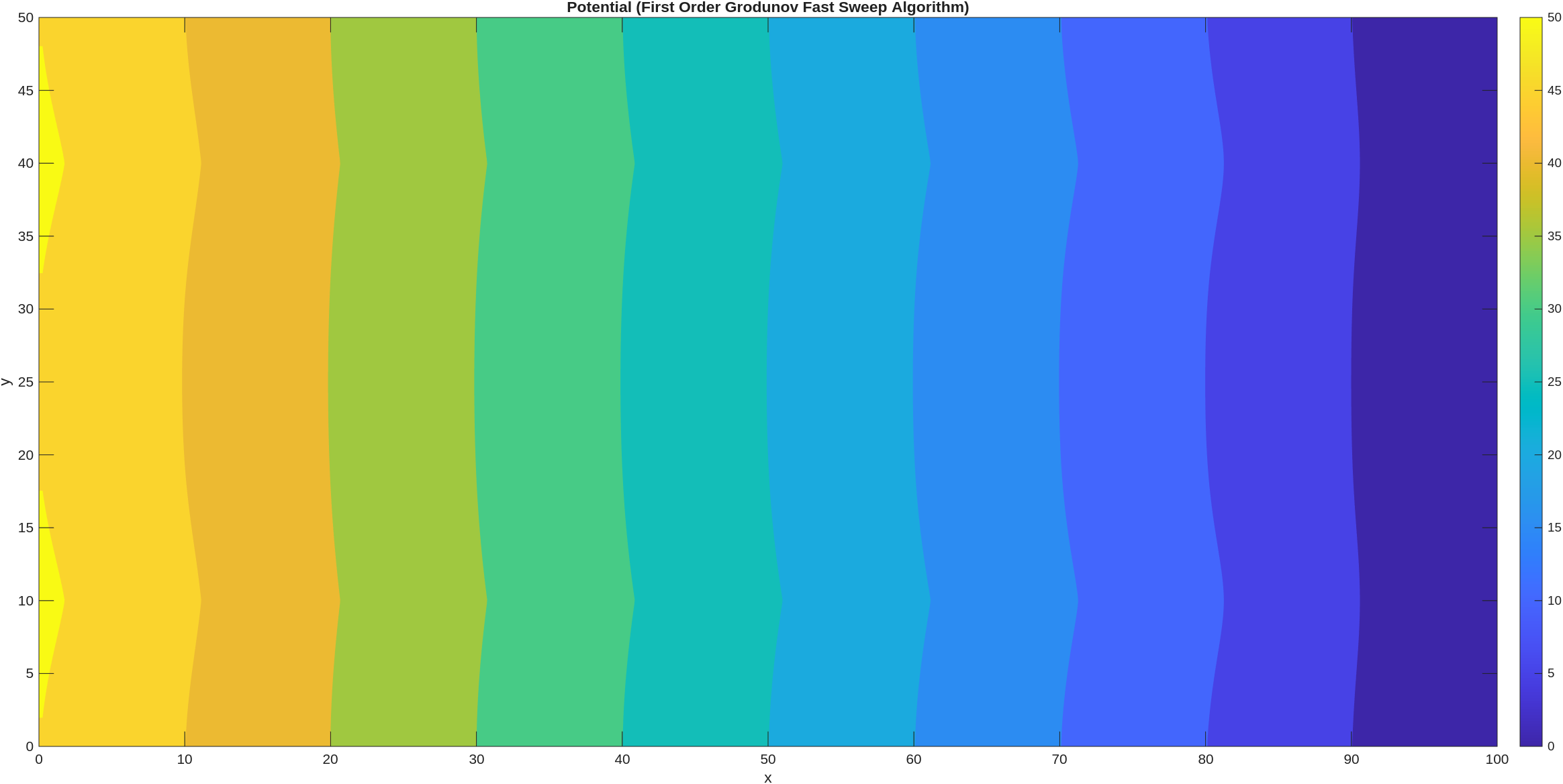
One crucial detail that I initially overlooked is that the paper initializes the value of phi using the solution obtained from an algorithm I had designed in the previous semester: the first-order Godunov fast sweeping method. This turned out to be a significant observation. Another important detail stated in the paper is that "for grid points whose distance to the boundary is less than or equal to 2h, the solution values are fixed as the initial guess during the iterations." This insight was particularly revealing, given the amount of time I spent trying to make the algorithm work. The choice of 2h also explains why the overall scheme achieves fifth-order accuracy.
The good news is that I have successfully implemented both the fifth-order WENO fast sweeping method and the fifth-order WENO advection scheme. However, I am still facing an issue. The approach I followed is described below.
1D Eikonal using 5th order WENO Fast Sweep
During a discussion with my professor, I was advised to begin by solving the problem in one dimension, which seemed reasonable. However, I faced a key difficulty: I was able to solve the one-dimensional fast sweeping problem for the crowd model because it was explicitly specified in the paper. In contrast, although the original Hughes paper first addresses the one-dimensional case before extending the analysis to two dimensions, I could not find a reference that described a one-dimensional fifth-order WENO fast sweeping method. As a result, I was uncertain whether this approach would work in practice.Nevertheless, I attempted to implement it, and the following report and code document my results.
As expected, this approach did not produce the desired results. This outcome is understandable, since designing an algorithm under the assumption that good performance in two dimensions will automatically translate to one dimension is flawed.
Two Dimensional Eikonal Equation
I therefore decided to retain the original objective of solving the two-dimensional Eikonal equation, which turned out to be a good decision, as it eliminated the need to work with a staggered grid; moreover, the WENO formulation of the Eikonal equation does not involve half-indexed terms such as i+1/2, making the algorithm straightforward to implement, and during this implementation I encountered two very important assumptions discussed in the paper.
- For higher-order nonlinear schemes (nonlinear due to the adaptive weights), the initial condition must be taken from the solution of the same problem computed using a lower-order scheme. This implies that the problem must first be solved using the lower-order method, which I had already implemented in the previous semester, and the resulting solution can then be used as the initial guess for the higher-order scheme.
- Another important observation was that the equality stated in the paper is incorrect. This error was the source of the complex-valued solutions I was obtaining. I had suspected this issue earlier—after comparing the formulation with the original fast sweeping paper—but initially assumed that the problem lay in my implementation. After multiple iterations, corrections, and verification, the program began to work correctly once the sign was changed, confirming that this was indeed an error in the published paper.
These were the observations, and the corresponding results are presented below. The following link provides the report for the two-dimensional Eikonal equation solved using the fifth-order WENO fast sweeping algorithm.

Two Dimensional Advection Equation
After successfully implementing the Eikonal equation, I proceeded to develop the code for the two-dimensional advection equation. This task proved to be more challenging than the Eikonal case, as it involved not only the WENO advection scheme but also the TVD Runge–Kutta time integration method. The WENO advection scheme is used to construct the semi-discretized form of the advection equation by discretizing the spatial derivatives.
This formulation requires the use of a staggered grid; however, to avoid unnecessary complexity, I did not explicitly define the staggered grid. Instead, it was handled internally within the relevant functions, rather than being defined and maintained globally. This design choice significantly simplified the implementation. In addition, I did not explicitly handle ghost points. The computational domain remains \(400 \times 200\), and the algorithm computes the solution only for indices \(4{:}N_x-2\), as required by the fifth-order upwinded scheme. As a result, the effective solution domain is \((N_x-5) \times (N_y-5)\); however, this compromise was acceptable given the substantial simplification it provided during implementation.
Provided below are the code and report for solving the two-dimensional advection equation using a fifth-order WENO scheme.
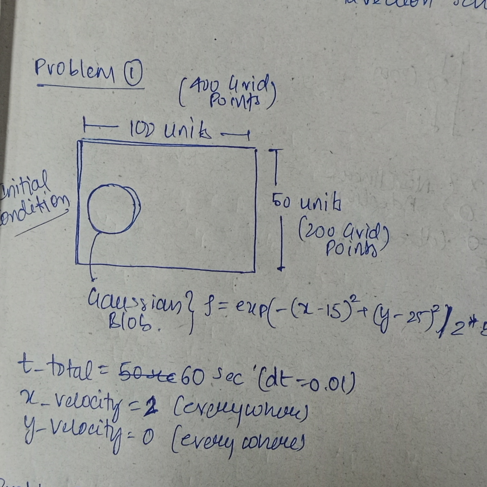
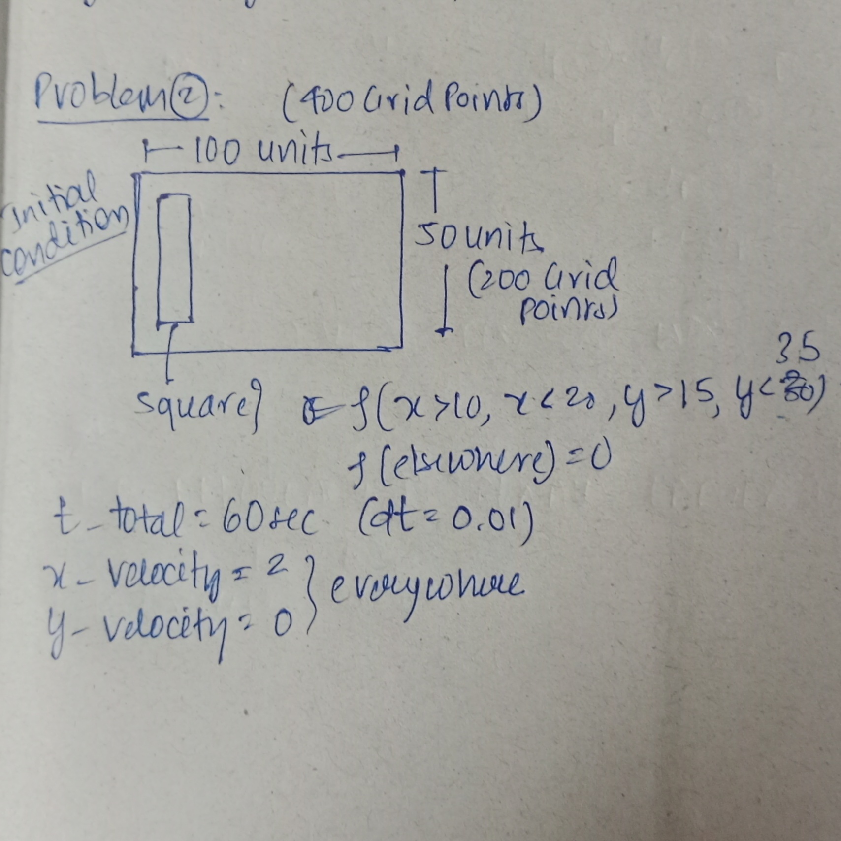
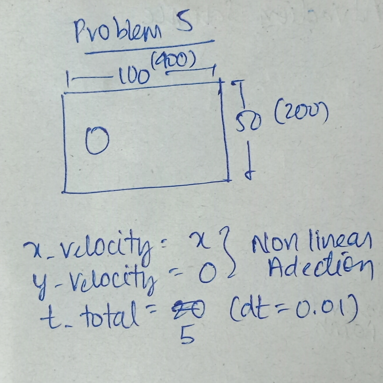
As shown in the results, two types of initial conditions and three types of test problems were considered. The first initial condition introduces a discontinuity in the density field (a square-shaped profile), while the second consists of a smooth Gaussian blob. The test cases include constant velocity in the x-direction (with no y-component), velocity components in both x and y directions, and a nonlinear velocity field. The nonlinear case, however, did not produce satisfactory results. The corresponding results are presented below.
| Problem | Initial Condition | Result |
|---|---|---|
| Problem 1 |
|
|
| Problem 2 |
|
|
| Problem 3 |

|
|
| Problem 4 |
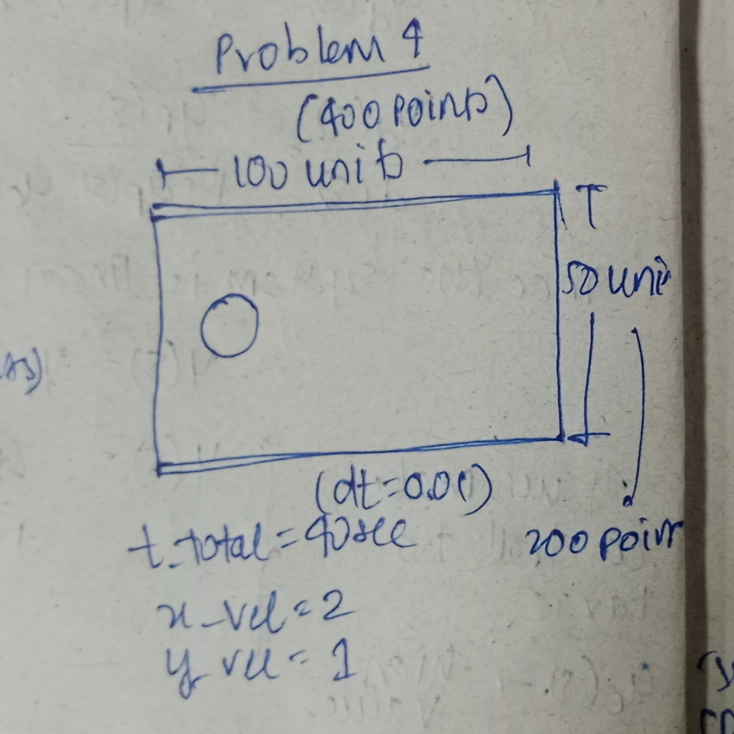
|
|
| Problem 5 |
|
I observe that the code becomes unstable when the velocity field is nonlinear, which is an issue I had mentioned earlier. This is precisely where I am currently stuck, since Hughes’ flow model involves a velocity field that varies spatially, making the advection equation nonlinear. Nevertheless, I attempted to use the same code framework to implement the Hughes’ flow model.
Two Dimensional Hughe's Flow
Using the successfully implemented Eikonal equation solver together with the problematic advection equation solver, I developed a solver for the Hughes’ flow model. As expected, the combined solver did not produce satisfactory results. The corresponding code, report, and results are provided below.
Presented below are the results for a synthetic test problem solved using the developed solver. As expected, the solution exhibits instability.
Meeting 11
Meeting 11
So after looking at the results of meeting 10, I was suggested to do the following.
- First is that I solved the advection equation with the velocity field that obeys the Greenshields' relation. Density vs X is plotted for Centerline constant Y values.
- Then I solved the problem of Hughes again with controlled delta_t (CFL) and with some modification in the boundary condition of the flux while solving the advection equation.
- Now, since the Hughes flow was facing a problem because of the new advection (higher order Advection), I have also tried solving the Hughes flow with my old advection solver, which used the first-order Lax–Wendroff equation, and also the newly formed Eikonal solver, which used a higher-order WENO fast sweep algorithm.
Old Eikonal and old Advection
So now I will be using the old eikonla and old advection solver to solve the same problem. And I am expecting to see no problmes making this code.
THis result of density could be used as soemthing to be looked forward to.
New Eikonal Equation solver and Old Advection Solver
Blunder
Here due to the advection equation being unstable for non linear advection equation, I have finally tried solving the problme with the old advection and new Eikonal Equation and here is the result
Density Distribution at Centerline
Density Distribution
Potential Distribution
Surprizingly what i noticed was that the results were still no good. And for this reason, I am re-attempting the problem with the old adection and old eikonal equation which I hav done in my last UGP. Here is the Report
Here is the corrected code. I have been making two blunders, and that is setting the inifnity value before the sweep to 10^2 which is very low. The paper recommeneded 10^12. And the second thing is I forgot the negative sign in the relation between the velocity and phi. Due to which i was getting some undesirable result shown in the above pop up.
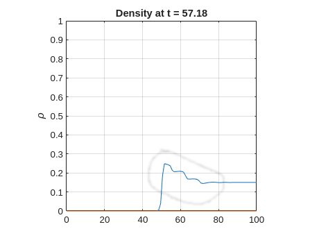
But after correcting the above blunder, I have finally generated a satisfoactory result using the new Eikonal and Old Advection equation, The Result for density is shown below. THis simulation of 50 sec took me almost an hour to process, hence the I havent increased the domain time. However it is obviousl that the simulation is not complete (Since not all the crowd have made it to exit in 50 sec).
And the result shows that new Eikonal Equation which is of the higher order is working as expected.
Non-linear Advection Problem with GreenSheild Relation
The last time I tried using the higher order Advection scheme (Fifth order WENO), I got the following result, which was for constant velocity.
For Constant Velocity Condition :The report for this code is given here : Report
It can again be seen that the Advection equation solver breaks for non linear problmes (Greensheild's velocity).
Hughes's Flow with the above Advection Equation
Blunder
Using the above Advection equation I againn tried solving the hughe's Flow problem, nad given below are the reuslts
After correcting a blunder this is the result for the problem with Higher order Eikonal and higher order Advection.
A Thought on Initial Condition
So in the quest of making the advection work, I tried lowering the initila condition. The reason was that when the density reaches the 0.5, then the image shown below occurs.
And so this time , I have first tried this initial condition on the 5th Order WENO Advection Equation, with varying velocity (GreenSheild's Relation). The problem description and the result for density is given below.
What I have seen here is that the density has changed advected but the way it does that is not as expected. I am suspecting that the problme is with the CFL value.
THe result given below are for the similar problem but solved usign the Lax Wendroff Scheme.
After finding that the advection solver worked some what better for lower veocity, I tried the same on the overall Hughe's Solver, and the problem description and the results are given below :
Meeting 12
Meeting 12
It has been a long time since I took over crowd dynamics. And in my last meeting, due to the advection equation causing problems, I was suggested to solve the 1D equation for the advection equation. The reason I think I directly started the 2D problem rather than first solving 1D and then moving to 2D was because I realised that the Eikonal Equation Solver (Fast Sweep method), but in WENO, discussed (and introduced to me) in the paper was in 2D. And since this method considered us to compare some quantities in the X and Y direction, I found it difficult to implement a WENO Fast Sweep without a concrete scheme mentioned somewhere. And the reason I was able to solve the 1D Fast Sweep in my previous semester was because the one dimensional Fast Sweep was already derived and mentioned in the previous paper that introduced the concept of the Fast Sweep (but not WENO, rather a simpler lower order method).
Also one more learning is that the explicit method to solve non-linear equations doesn't have to involve iteration, but for the implicit method it has to be iterative.
But since now I am not required to solve the 1D Hughe's flow completely (which requires me to know about the 1D WENO algorithm for both advection and eikonal), I can just solve the 1D advection using the WENO, fix the problem if any, and then directly use the learning from this to 2D advection and then fix it. And since my 2D eikonal solver with WENO is already working, I can then move on to solve Hughe's flow in 2D completely using the WENO. So that's an overview of all the work that I will be doing for this meeting. Moving on...
One Dimensional WENO Algorithm.
Problem :
Given below is the code, and here is the report :
Problem Description :
Code
clc;
clear all;
%-------Domain Parameter-----%

% Grid Points

global Nx;
Nx = 400;

%--Important Parameters--%

INFINITE = 10^12;
global eta; eta = 10^-6;
error_eta = 10^-9;
CFL = 0.5;

% Dimension of Domain
Lx = 100;

% Domain
x = linspace(0,Lx,Nx);

% Defining velocity
global x_velocity;

% Space Interval
global h;
h = Lx/Nx;

% Total Time
t_total = 150;
Initial Condition (Density and Velocity)
% -- Initial Condition (Density) -- %

xc = 15;     % center x
sigma = 5;   % width
rho = 0.2*exp(-((x-xc).^2) / (2*sigma^2) ) + 0.1;

% -- Initial Condition (Velocity) -- %
%--Function to compute Velocity using Density

function speed = makeSpeed(rho)

    global Nx;
    speed = zeros(1,Nx);

    for i = 1:1:Nx
        speed(1,i) = 1 - rho(i);
    end

end

x_velocity = makeSpeed(rho);
Flux Calculation
% -- Function that will calculate the flux depending on the u,v and Density -- %
function flux = makeFlux(rho)

    global Nx x_velocity;

    % Initialzing Flux
    flux = zeros(Nx);

    for i = 1:1:Nx
        flux(i) = rho(i) * x_velocity(i);
    end

    % Assign the boundary flux to be equal to zero
    flux(1) = 0;
end
Time Marching
%--Preallocating the memory
rho_n = zeros(Nx);
rho_1 = zeros(Nx);
rho_2 = zeros(Nx);
rho_next = zeros(Nx);


%-----------MAIN SOLVER------------%
t = 0;
step = 0; % For plotting at regular interval


while t< t_total

    % Computing Cost For the density rho
    x_velocity = makeSpeed(rho);

    % Updating the delta_t with proper CFL condition (Wiki Pedia)
    u_max = max(x_velocity(:));
    dt = CFL / ( u_max/h + 1e-12 );

    % -- Making rho_n and RHS of rho_n
    rho_n = rho;
    semi_discritze_form_rho_n = makeRHS(rho_n);


    % ---------- Making the RHO_1 and then RHS of rho_1 ------ %
    for i = 4:1:Nx-2
        rho_1(i) = rho_n(i) + dt * semi_discritze_form_rho_n(i-3);
    end

    % -- Extrapolation (My Intuition)
    rho_1(3) = rho_1(4); rho_1(2) = rho_1(3); rho_1(1) = rho_1(2);  % Right Edge
    rho_1(Nx-1) = rho_1(Nx-2); rho_1(Nx) = rho_1(Nx-1);             % Left Edge

    % -- RHS of discritised form using rho_1
    semi_discritze_form_rho_1 = makeRHS(rho_1);


    %--------- Making the RHO_2 and RHS of RHO_2 ----------%

    for i = 4:1:Nx-2
        rho_2(i) = 3/4 * rho_n(i) + 1/4 * (rho_1(i) + dt * semi_discritze_form_rho_1(i-3));
    end

    % -- Extrapolation (My Intuition)
    rho_2(3) = rho_2(4); rho_2(2) = rho_2(3); rho_2(1) = rho_2(2);  % Right Edge
    rho_2(Nx-1) = rho_2(Nx-2); rho_2(Nx) = rho_2(Nx-1);             % Left Edge

    % -- RHS of discritised form using rho_2
    semi_discritze_form_rho_2 = makeRHS(rho_2);


    %----------Making the rho_next-------------------------%

    for i = 4:1:Nx-2
        rho_next(i) = 1/3 * rho_n(i) + 2/3 * (rho_2(i) + dt * semi_discritze_form_rho_2(i-3));
    end

    % -- Extrapolation (My Intuition)
    rho_next(3) = rho_next(4); rho_next(2) = rho_next(3); rho_next(1) = rho_next(2);    % Right Edge
    rho_next(Nx-1) = rho_next(Nx-2); rho_next(Nx) = rho_next(Nx-1);                     % Left Edge

    step = step + 1;

    %--Plotting rho
    if mod(step,1) == 0

        figure(6);
        plot(x, rho, '-');   % blue line with thickness

        ylim([0 1]);
        xlim([0 100]);

        title(sprintf('Density at t = %.2f', t));
        xlabel('x');
        ylabel('\rho');

        grid on;
        axis square;

        drawnow;

        frame = getframe(gcf);
        writeVideo(video, frame);

    end


    % Substituting back the rho value \
    rho = rho_next;

    % Updating the time
    t = t + dt;
end
Semi Discrete form
function semi_discrete_form =  makeRHS(rho)

    global Nx x_velocity h;
    semi_discrete_form = zeros(Nx-5);

    %--Flux for the given rho distribution
    flux = makeFlux(rho);

    % Calculating the maximum speed
    alpha_x = max(x_velocity(:));


    % -- Calculating the value of f+ and f- at {i+2,i+1,i,i-1,i-2,i-3} -- %
    fx_negative_whole = zeros(Nx);
    fx_positive_whole = zeros(Nx);

    for i = 1:1:Nx
        fx_positive_whole(i) = 1/2 * (flux(i) + alpha_x*rho(i));
        fx_negative_whole(i) = 1/2 * (flux(i) - alpha_x*rho(i));
    end

    % -- Computing the RHS of Semi Discrite form.
    for i = 4:1:Nx-2

        %--X--%

        % fx{+}_[i+1/2,j]
        fx_plus_x_half_forward = stencil( ...
            fx_positive_whole(i-2), ...
            fx_positive_whole(i-1), ...
            fx_positive_whole(i), ...
            fx_positive_whole(i+1), ...
            fx_positive_whole(i+2));

        % fx{+}_[i-1/2,j]
        fx_plus_x_half_backward = stencil( ...
            fx_positive_whole(i-3), ...
            fx_positive_whole(i-2), ...
            fx_positive_whole(i-1), ...
            fx_positive_whole(i), ...
            fx_positive_whole(i+1));

        % fx{-}_[i+1/2,j]
        fx_minus_x_half_forward = stencil( ...
            fx_negative_whole(i+2), ...
            fx_negative_whole(i+1), ...
            fx_negative_whole(i), ...
            fx_negative_whole(i-1), ...
            fx_negative_whole(i-2));

        % fx{-}_[i-1/2,j]
        fx_minus_x_half_backward = stencil( ...
            fx_negative_whole(i+1), ...
            fx_negative_whole(i), ...
            fx_negative_whole(i-1), ...
            fx_negative_whole(i-2), ...
            fx_negative_whole(i-3));

        fx_positive_half = fx_plus_x_half_forward + fx_minus_x_half_forward;
        fx_negative_half = fx_plus_x_half_backward + fx_minus_x_half_backward;

        %--Boundary Condition -- %

        % Left Wall (Flux set to Zero)
        if(i == 4)
            fx_negative_half = 0;
            fx_positive_half = 0;
        end

        % Right Wall (Flux Set to Zero)
        if(i == Nx-2)
            fx_positive_half = fx_positive_half;
            fx_negative_half = fx_negative_half;
        end

        % Computing RHS of Semi Discritized form
        semi_discrete_form(i-3) = - 1/h * (fx_positive_half - fx_negative_half);
    end
end
Stencil
% To compute f half. Order of input matters
function f = stencil(f1,f2,f3,f4,f5)

    global eta

    % Compute S values
    s_1 = ((1/3) * f1) + ((-7/6) * f2) + ((11/6) * f3);
    s_2 = ((-1/6) * f2) + ((5/6) * f3) + ((1/3) * f4);
    s_3 = ((1/3) * f3) + ((5/6) * f4) + ((-1/6) * f5);

    % Compute Beta
    beta_1 = 13/12 * (f1 - 2*f2 + f3)^2 + 1/4 * (f1 - 4*f2 + 3*f3)^2;
    beta_2 = 13/12 * (f2 - 2*f3 + f4)^2 + 1/4 * (f2 - f4)^2;
    beta_3 = 13/12 * (f3 - 2*f4 + f5)^2 + 1/4 * (3*f3 - 4*f4 + f5)^2;

    % Definign Gamma
    gamma_1 = 1/10;
    gamma_2 = 3/5;
    gamma_3 = 3/10;

    % Computing weights bar
    w_1_dash = ( gamma_1 ) ./ ((eta + beta_1)^2);
    w_2_dash = ( gamma_2 ) ./ ((eta + beta_2)^2);
    w_3_dash = ( gamma_3 ) ./ ((eta + beta_3)^2);

    % Computing Weights
    w_1 = ( w_1_dash ) / (w_1_dash + w_2_dash + w_3_dash);
    w_2 = ( w_2_dash ) / (w_1_dash + w_2_dash + w_3_dash);
    w_3 = ( w_3_dash ) / (w_1_dash + w_2_dash + w_3_dash);

    % Computing Flux
    f = w_1 * s_1 + w_2 * s_2 + w_3 * s_3;

end
And here is the results:
I see that the solution is still very oscilatory. It could be possible that this is the solution. The solution that I got from my previous model for this problem is given below :
I have thought to give the paper of the WENO advection, a reading. And then I think I wil continue with the implementing the one dimensional Advection using WENO. And this will take some time. Given below are the list of websites and alsoa paer, that i am reading to understand the WENO algorithm.
Meeting 13
From my previous conversation, I had the following suggestion. Here is this attempt. I am going to do the following.
- First get the results for the one dimensional advection equation using the WENO
- Then get the velocity to be equal to some function of (X) rather than being a function of density
- And then make the gradient of the initial condition of the density smoother
1. Constant Velocity Distribution:
For the purpose of my toy problem, in all my attempts of solving this problem, I have taken the ghost points to be Nx = 0, Nx = 1, Nx = 2, Nx = 3 and Nx = 399, Nx = 400.
Parameters
- Constant velocity everywhere: u(x) = 10
- Center of the blob is at Lx = 20 units (Nx = 80)
- CFL = 0.5
- Total time: 10 units
- Boundary condition is fi-1/2 = 0 at i = 4. And the rest of all the values of f at the ghost points are never computed. However, the values of density are extrapolated.
Velocity expression and the result are given below.
2. Spatially Varying Velocity:
So now I have made the velocity to be just a function of space. And the expression for the velocity is given below.
The reason I have taken 0.1 is because I wanted to keep the maximum velocity not very high. Hence, the X coordinate has to be scaled down. Since the constant velocity is 10, it is because I have seen that the solution is somewhat more stable compared to when all the velocity comes from the linear part alone. So in a way, I am making the velocity the sum of a linear and a constant component.
Rest of all the parameters are kept the same.
Green Shield's Relation
Now I have finally made the Greenshield's relation, but there is one difference, and that is that this time, I have taken the velocity to be the sum of constant velocity and the Greenshield. (Just like in the above case, where the velocity is the sum of constant and linear velocity component). Parameter is kept the same.
One paper that I was interested in was the this. At soem poijt will also try understandign it, since it solves the same problem as that which I am tryign to solve, and maybe it migt have better explanation compared to my present paper.
Meeting 14
So one important suggestion that I got from my professor is as follows:
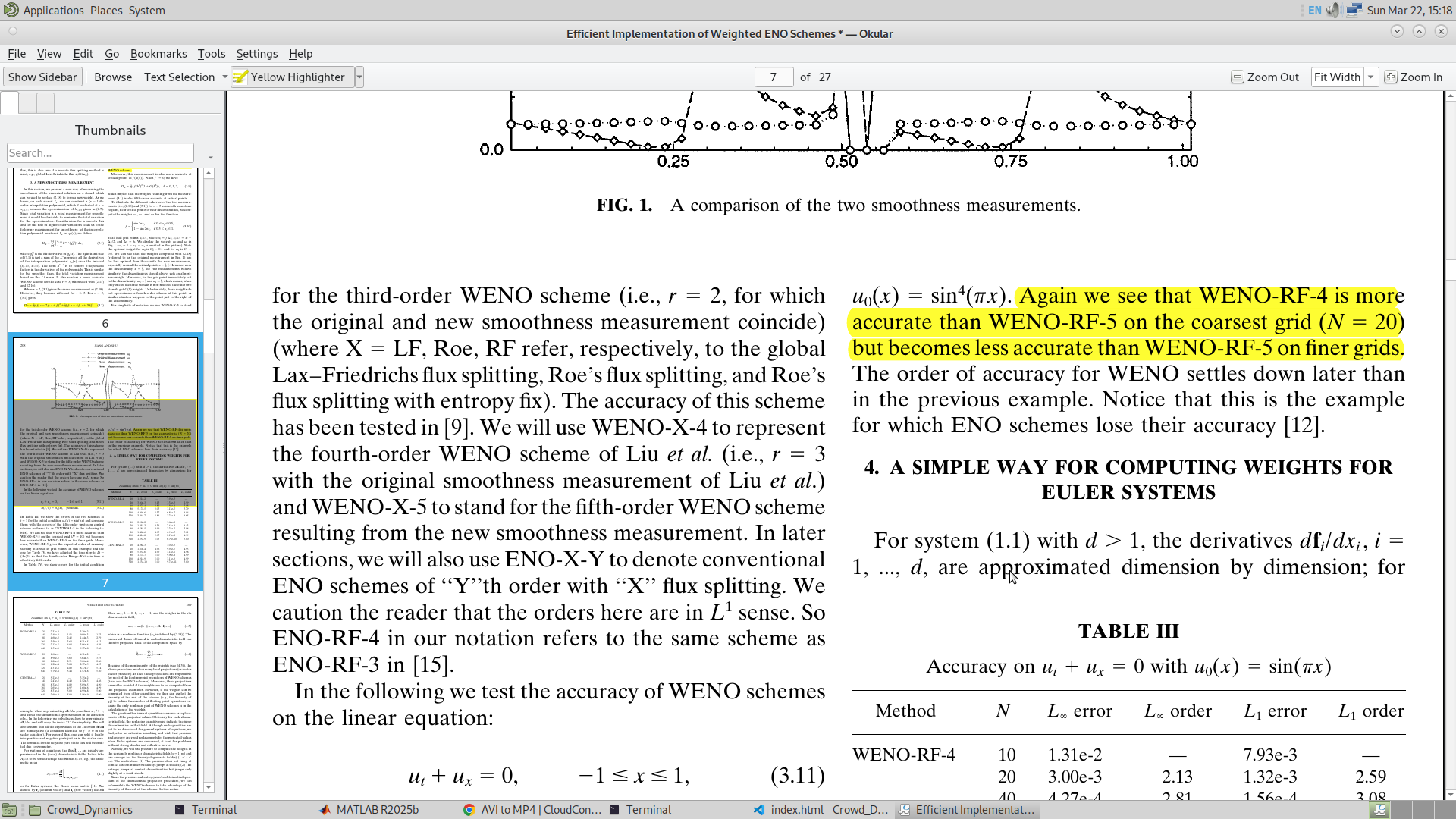
In my previous attempts, I almost missed this very subtle point that was also mentioned in the paper. And that was that this scheme of WENO was made to solve the problem on a grid size of 100×50 for the actual domain dimension of 100×50. Which means the space interval dx and dy is equal to 1. But I was rather solving it on a (400×200) mesh with the space interval being 0.25.
The actual abstract from the paper is given below, which shows that WENO is solved on a coarser mesh.
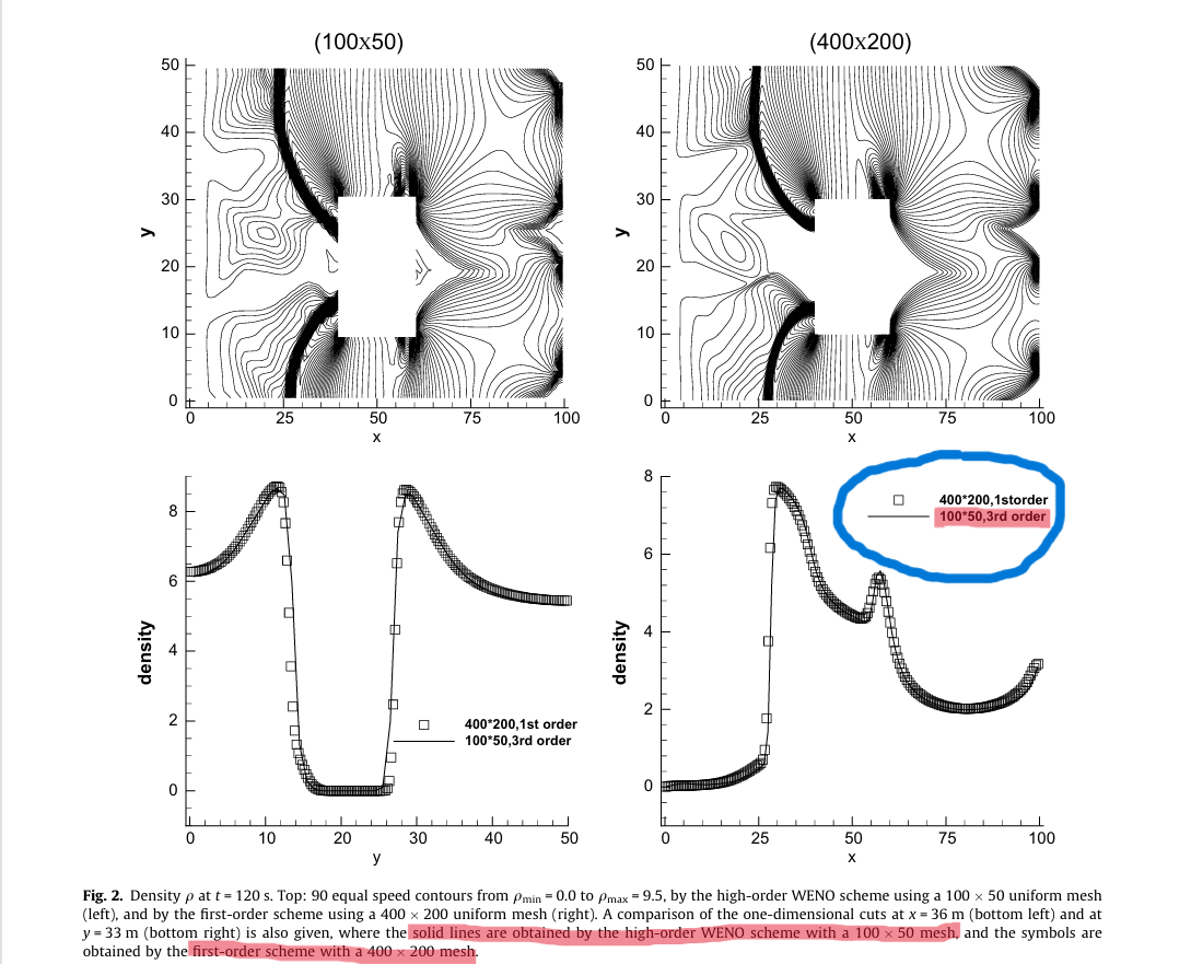
Because of me being careless, I never thought that the author might solve the scheme on a coarser mesh. What I expected was that a finer mesh is always a good thing to have. But this was unexpected.
In the discussion with my professor, he also showed me that this was mentioned in the original paper of WENO as well. And since I never expected this problem to arise in the first place, I missed seeing this detail in the original paper too. Given below is the part of the original WENO paper that explains this.
One Dimensional Advection WENO Solver :
This is the problem statement for my one diensional problem :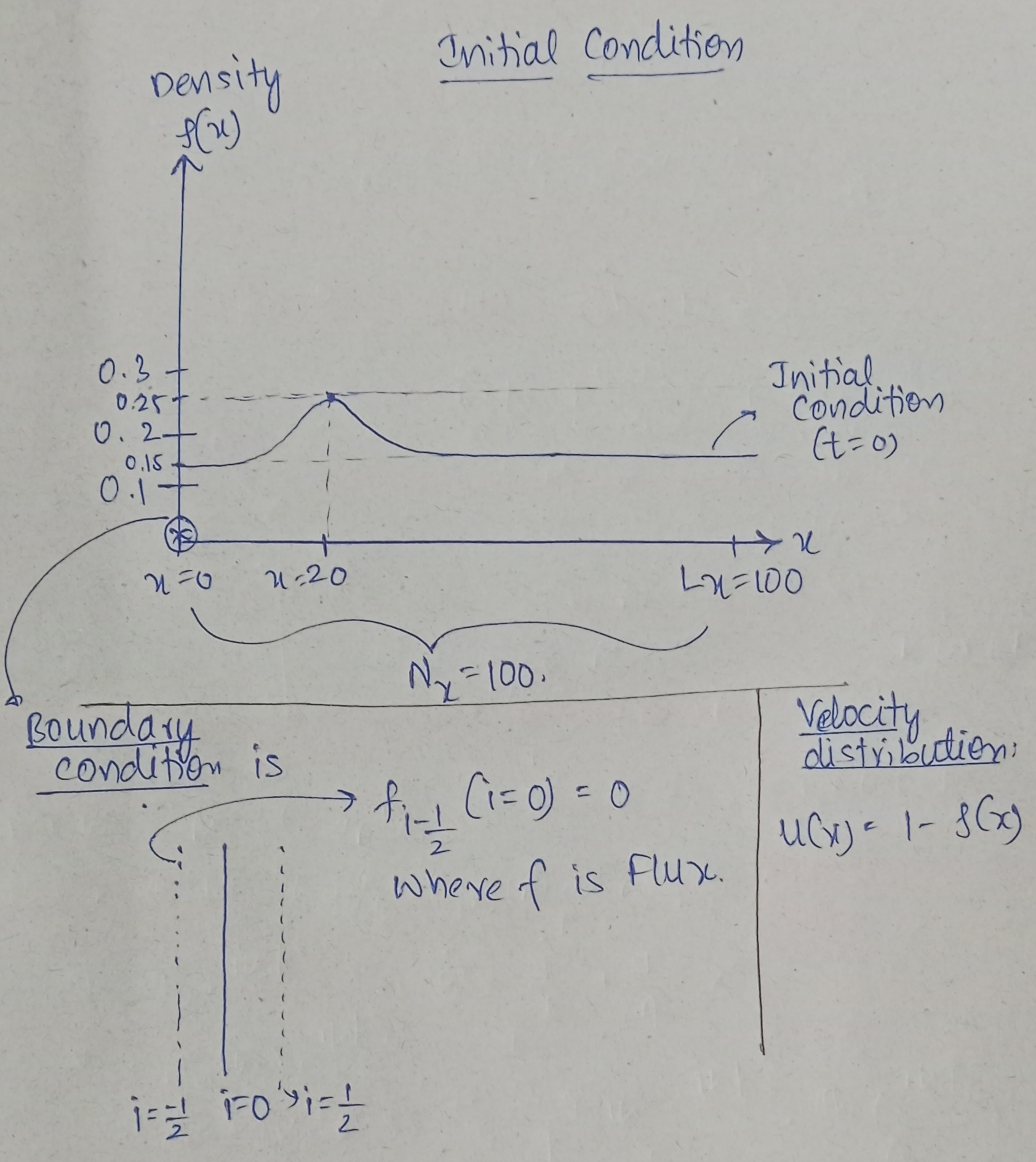
So finally, with that being said, this is the result I got for the problem I am solving.
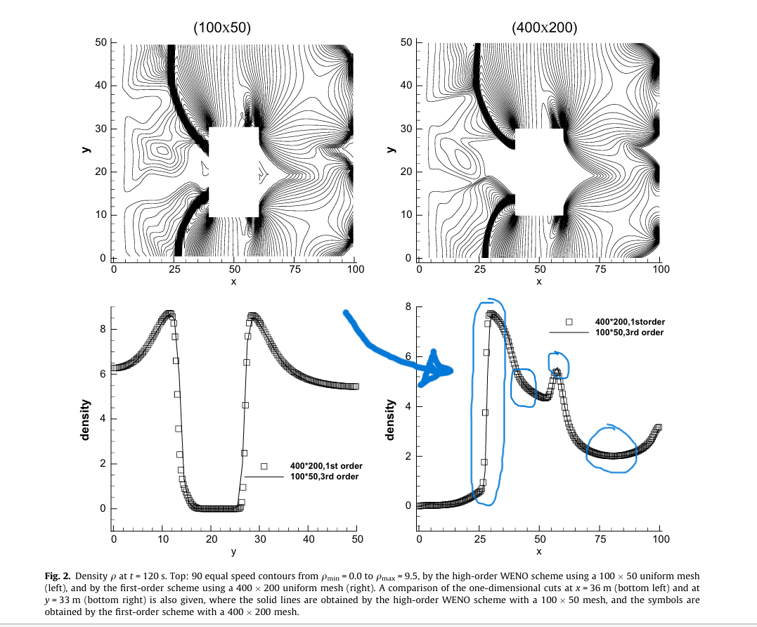
The results are actually good. Because when seeing this, I can observe that the solution does contain shocks, but there are bumps in the solution (infront of the shocks). Now these bumps are also something I have seen in the original Railway Station paper, and this gives me some relief. It might be possible that all my problems boil down to having a finer grid. The solution to this would be to use a coarser mesh. Amazing...
Given below is the solution of the original paper, and my solution side by side.
Here is the Report and the Code for the above one dimensional problem.
Two Dimensional Advection WENO Solver :
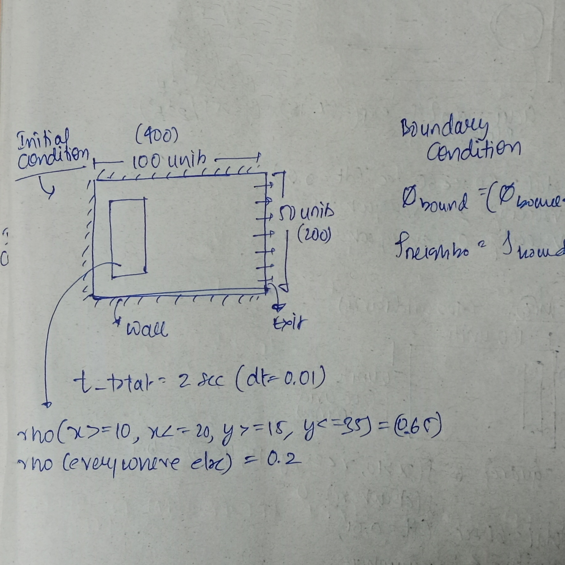
Now with the understanding on the one dimension, I am going ot solve the problem of advectino equation, but with two dimension. And the problem statement is given below.I have with me the problem where there is wall in all the three sides (Top, Bottom, and Left), and there is outflow of crowd at the right side of the domain. And there is a gaussian blob at some location in the domain. And this will be advected in the domain. The boundayr condition that I ahve imposed is as follows.
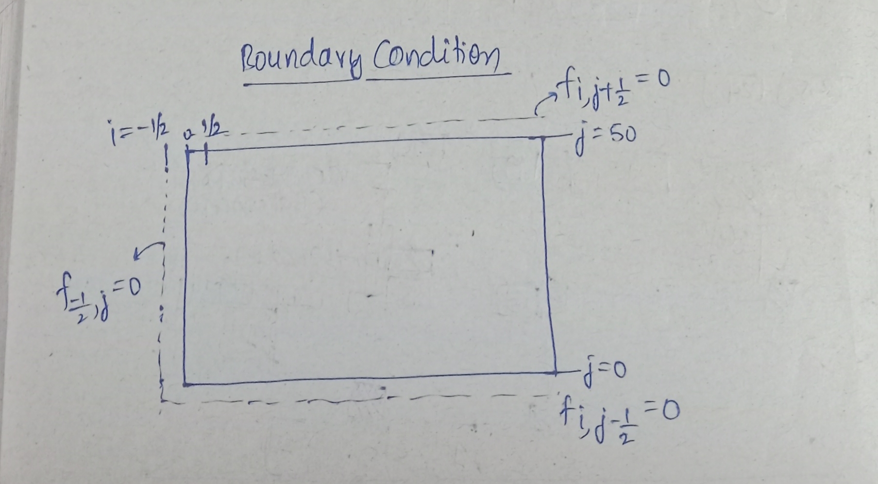
At the boundary the normal flux at the staggered grid just inside the non-staggered grid is equalk to zero. Which mean at right boundary (let say at x = 0), the x-flux at x = 0 - 1/2 is equal to zero. Similarly at the bottom boundary where the cordinates of the y = 0, the value of flux f at y = 0 - 1/2 is equal to zero. And similary at the top boundary where y = 200 I have set the y-flux at y = 200 + 1/2 to be equal to zero.. The pictorial representation of the same is given below :
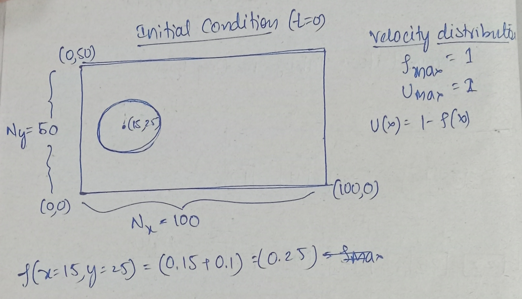
Anbd here is the initial condition :
And the results are given below :
I do see some discrepancy, like the solution giving some nonsensical results at the x~46 units but apart from that the solution does look good. There are shocks forming at the edges signifying that the crowd behind with higher velocity is pushing the crowd at front wiht lower velocity. here is the Code and Report.
Two Dimensional Hughe's Flow :
Given below is the description of the problem, and I will be trying to solve using the Hughe's Flow and the advection and Eikonal Equation that I will be solving.
I have tried solving it, and here is the result I got from that. I see that the solution again blew up.
Here is the Report and the Code of the above results for the Hughe's Flow.
References
- A continuum theory for the flow of pedestrians (Original Paper on the Hughe's Pedestrian Flow)
- Revisiting Hughes’ dynamic continuum model for pedestrian flow and the development of an efficient solution algorithm (Paper with Railway Station Problem)
- Capturing stochastic variabilities in pedestrian flows: A dynamic continuum modeling approach (Paper solving the same railway station problme but with some other method)
- A FAST SWEEPING METHOD FOR EIKONAL EQUATIONS (Original Ppaer on the Fast sweep)
- Efficient Implementation of Weighted ENO Schemes (Original paper on the WENO)
- Brief of finite volume WENO method (An interpretation on the WENO method)
